DOWN HOLE SEISMIC FOR ENGINEERING STRUCTURES

I. INTRODUCTION

1.1. General  Statement

Applied seismic on engineering structure divided into 2 (two) advantages, that are:

Firstly, refraction seismic exploration is to get lateral distribution of velocity layers underneath ground level. The velocity layers related to bearing capacity of soil or rocks. Beside that, the velocity layers could be known unconsolidated material and solid rock, depth of soil or base rock. Others, usefully of seismic exploration are to reduce core drilling in feasibility stage engineering study.

Secondly, down hole seismic is to get bearing capacity parameter in relation to engineering structure when the earthquake happened. The method to do down hole seismic is to install geophones on the bore hole, than making artificial trigger on the surface. The impulse or artificial trigger can be rise compression wave and shear wave. The result of preliminary wave and the secondary wave can be use to get the dynamic characteristic of the soil or rocks.

The result of the applied seismic given to engineer for designing the resistance of earthquake on engineering structure.

1.2. Basic Theory

In the seismic refraction method an explosive charge, weight drop or hammer blow is used to generate an elastic pulse (shot) at the earth’s surface. Some of the radiating energy which travels by several paths in the medium is refracted along subsurface boundaries and returns to surface to be recorded by a line of detectors (seismometer or geophone). The time lapse between the shot and the first arrival of the refracted energy at each of geophone is plotted on the time-distance curve (Fig.1) and this provides information on the depths to the refracting horizons and the seismic velocities of underlying layer. Fortunately, refracting horizon normally corresponds to distinct geological horizons and thus the depths to the geological interfaces may be computed. Modern interpretation techniques permit the measurement of depth to an irregular refracting interface at each seismometer position along the profiles.

1.3. The Down Hole Seismic

The purpose of down hole seismic is to be able to predict with accuracy behavior earthquakes of structure and the ground on which its rest, and used for effective a seismic design. It is necessary to know the dynamic characteristics of the ground.

The dynamic characteristics of soil that must be known in order to analyze deformation and stress resulting from dynamic loads are the Poison’s ratio (α), shear modulus (G), Young’s modulus (E) and kinetic bulk density (K).  

Those parameters can be calculated using the formula as shown bellows:

Kinetic Poisson ratio’s                      α = {1 – 2 (Vs/Vp) ²} / {2-2(Vs/Vp) ²}

Kinetic Rigidity Modulus                 G = 1/g.r.Vs² (in kg/cm²)

Kinetic Deformation Coefficient      E = 2(1+r) G (in kg/cm²)

Kinetic Bulk Modulus                       K = E/3(1-2r) (in kg/cm²)

Where             g = acceleration from gravitation (9.75 m/sec²)

                        r = bulk density of the ground (tonf/m³)

                        Vs and Vp = seismic velocity (m/sec)

The primary wave (Vp) and shear wave (Vs) is known from the down hole seismic record.

CHAPTER 2. PROCEDURE OF DOWN HOLE SEISMIC

The three of geophones is inserting to the bore hole as shown in Fig.2. The length of prove is 1.00 m, where on the tip of prove contained three geophones perpendicular each others.

The P wave and S wave propagation determine by using 3 geophones, 1 geophone placed vertical and two geophones horizontal. The two geophones placed on the right angles to each others. The shot point is toward the hole about 1.50 m – 2.00 from the hole. The wooden plate hammering is method to generate shear wave referred to every depth of hole. 

The wooden plate is 1.50 m – 2.00 m long, 50 cm wide and 10 cm thickness is firmly fixed on the ground. The data will be checked for be sure measurement of S waves. The record will be every 1 m interval and the record similar up to the depth of hole. The V wave and S wave determined from the record and plotted on the paper to determine of velocity layers.

Figure 2. Schematic Down Hole Seismic using the Oyo Mc Seis 160. 

2.1. Calculation of Dynamic Parameter

The down hole seismic method is applied to find the velocity distribution of P wave and S wave in bore hole. The first step of finding velocity distribution is to read the first arrival time on the seismic record. Afterward, data is plotted on the millimeter paper and drawing the time - travel curve. On the curve find the best fit of velocity distribution (Vp or Vs= distance / time = m/sec.)

The velocity distribution of P wave and S wave are used to calculate the dynamic elastic constant as shown on the flow chart on Table 1.

Table 1. Processing to produce dynamic elastic constants from S wave and P wave (OYO, 1978, TN 18).

P wave velocity is chiefly a function of volume elasticity and rigidity of the layer, become smaller in rigidity in proportion as the layer is soft with result that volume elasticity comes to have a larger influence.

S wave velocity, which is function of only rigidity, is a volume which serves s direct standard of hardness of layers. The values of material density (r) is obtained from Table 2.

Table 2. Density values (r), angle of friction (φ⁰), compaction (C) according to JIS Manual.

Material types	Rock types	Unit Weight (r) (tf/m3)	Angle of friction (φ0)	Compaction ( C ) =kgf/cm2	Soil Classification
Banking Material		1,4 – 2,0	150 - 400	0,1 – 0,5	GW,GP SW,SP SM,SC ML,CL VH
	Gravel	2,0 1,8	40o 35	0	GW,GP
	Sand with gravel	2,1 1,9	40 35	0	GW,GP
	Sand	2,0 1,9	35 30	0	SW,SP
Natural	Sandy soil	1,9 1,7	30 25	0	SM,SC
Material	Clayey soil	1,5 1,6	25 20	0	ML.CL
	Clay and silt	1,6 – 1,7 1,4 – 1,5	20 15	0	ML.CL MH
	Volcanic ash	1,4	5	0,3	VH

CHAPTER 3. THE RESULTS OF DOWN HOLE SEISMIC

The time travel curves and elastic modulus shown on Table 4 and Table 5. The elastic modulus related to the depth of ground bed design and the weight of proposed engineering structure. The summary result of down hole seismic shown on Table 3.

CHAPTER 4. CONCLUSIONS

Elastic modulus taken from the data of AR 1 on the depth of 15 m is as follows :  

α    = 0.33 – 0. 50

G   = (0.2 x 10³ – 189.9 x 10³) kg/cm²

E   = (1.34 x 10³ – 1025.34 x 10³) kg/cm²

K   = (41.22 x 10³ – 483.50 x 10³) kg/cm²

r    = 1, 7 – 1, 8    

REFERENCES

1.    Masuda, H., 1975, Seismic Refraction Analysis for Engineering Study. OYO Technical Note TN 10.

2.    Imai, T., 1975, An Introduction to the geophysical prospecting for civil engineering purposes. OYO Technical Note TN 11.

3.    Hawkins, L.V., 1961. The reciprocal method of routine shallow seismic refractions lines. Geophysical Prospecting, 6, 285 -182.

4.    Hawkins, L.V., 1961. Seismic Refraction Surveys for Civil Engineering. Geophysical Memorandum 2/69, ABEM Printed Matter No.90091.

5.    Angela M. Davis, 1977, A Technique for Insitu Measurement of Shear Wave Velocity, Marine Science Laboratories, University Collage of North Wales U.K,, Abem  Case History, ABEM Printed Matter – No.90180

6.    Takeshi Okubo, Akhiro Satake, Masaki Ishoguro, Minuro Nakagawa and Ken Ito, 1978, Seismic Survey for Civic Engineering by Handy Seismograph, OYO Technical Note TN – 18, OYO Corporation. 

 7.Satoru Ohya, Tsuneaki Takeuchi, Tsuneo Imai and Ken Ito, 1978, Geophysical Investigation for Civil Engineering purposes in Japan. OYO Technical Note TN – 33 OYO Corporations.

RESISTIVITY REPORT FOR SHALLOW GEOTHERMAL AT MARGA MUKTI, KECAMATAN PANGALENGAN, KABUPATEN BANDUNG SELATAN, PROVINCE OF WEST JAVA

    

RESISTIVITY REPORT

FOR SHALLOW GEOTHERMAL AT MARGA MUKTI, 
KECAMATAN PANGALENGAN,

KABUPATEN BANDUNG SELATAN,

PROVINCE OF WEST JAVA

ABSTRACT

The geoelectric sounding have been carried out at the hot spring Desa Marga Mukti, Pangalengan, Kabupaten Bandung Selatan. The geoelectric sounding has been done into 2 (two ) sounding way , first to do geoelectric sounding 1-D with electrode arrangement of Schlumberger. The second geoelectric sounding was the resistivity 2-D with electrode arrangement Wenner-Schlumberger on the same line. The results of the both sounding was the values of resistivity 2-D  lower than the resistivity 1-D. the area is covered by the rock unit which is contained water bearing formation . Those water bearing formation partly influent on the heating rocks or hot fluid, so the water bearing formation divided into saturated rock with fresh water and hot water. The value of the hot water is between 0.32 ohm-m to 7.29 ohm-m. It is caused that the hot fluid or heating rocks having water temperature increase  and the resistivity of fluid is decreases. This is caused the lower viscosity and higher mobility of ions, so the resistivity value became lower. The resistivity of hot fluid was  between 0.1 ohm-m to 10.0 ohm-m.      

1.   INTRODUCTION

Generally ,the geothermal system in Indonesia is a hydrothermal system with high temperature ( > 225⁰ C) and on the several places have low temperature (150⁰-225⁰C ). The hydrothermal system created by results of heating movement  from the sources to surrounding areas with the conduction and convection heat current. The movement hot fluid with conduction through rocks, however the movement hot fluid with convection current caused contact  between the fresh water and hot fluid.

The indication of hydrothermal system in underground could be seen from geothermal surface manifestation, such  as hot water or hot water spring, mud pools water and geyser. The geothermal manifestation on the surface is assumed the transmission of hot movement from the underground  or existed of fractures , which is hot fluid flew to the surface.       

Geoelectric sounding could be carried out to know contrast distribution of resistivity of fresh water and hot fluid water. The consideration of the geoelectric sounding as described belows :

1.1.    RESISTIVITY OF WATER SATURATED

DC Resistivity method has proved to be a useful tool in the exploration geothermal. Water dominated geothermal systems usually have a lower resistivity than the surroundings colder rocks, whereas vapor dominated systems may be characterized by high resistivity. The resistivity of rocks is controlled by severals parameters , which will be deal with the following section.

1.1.1.   The texture and porosity of the rocks.

In general dry , coarse crystalline rocks have a high resistivity, but fine grained clays, highly vesicular and altered rocks as well as alteration products show a low resistivity. Usually the water has a lower resistivity then the rock matrix itself and is the dominant factor in the resistivity of the rock as  a whole. This correlation can be expressed by Archie’ Law ( Keller and Frischknecht, 1966 ) :

                                    ρ= a . ρ_w  . φ^-m                             ( 1 )

where ;

ρ    = the bulk measured resistivity of water saturated rock

ρ_w   = the resistivity of water filling the pores ;

φ  = the fractional amount of porosity in corrosion with the total volume;

a    = a constant which is less than 1 for inter granular porosity and higher than 1.

m = the cementing factor which varies from 1.2 or unconsolidated sediment to 3.5 for crystalline rocks;

As first approximation the values a = 1 and m = 2 are used.

Equation ( 1 ) indicates that ratio ρ/ ρ_w higher  is a constant for given porosity . This relation can be expressed by the formula :

                                    F = a . . φ^-n                                           ( 2 )

where F is formation factor.

1.1.2.     The Salinity of the Water

The salinity of the water ( liquid ) present in the pore space of the rock effects the resistivity of the bulk rock. We can look upon the water as an electrolyte. The conductivity of an electrolyte solution can be expressed  by :

O = 1/ρ= F (C₁ . m₁  +  C₂ . m₂  + C₃ .m₃ ......)              (3 )

where  m₁ = mobility of moving ion

             C₁ = concentration of ions

             F = Faraday number  ( 96500 Coulombs )

The concept of an equivalent salinity is usually used in explaining the resistivity of groundwater. The equivalent salinity of solution is defined as the salinity of a NaCl solution having the same resistivity as a solution containing various salts.

The advantage of using equivalent salinity is that only one table ( or graph ) for a single salt is needed to determine the resistivity of a solution. The curves showing the relation ship between the resistivity and the salinity of NaCl solutions at various temperatures are shown in Fig. 1.

The figure 1 shows that there is an element linaer relationship between the salinity and the conductivity of electrolyte solutions. For t = 0⁰ C the relation between the salinity of the resistivity can be determined by the equation ρ = 0.211 x C – 0.937 where the resistivity (ρ ) is in ohm-meters and C in mol ( 1 mol = 58450  ppm )

Figure 1. The relationship between the resistivity of a NaCl solution and the salinity of the electrolytic solution of the different temperature ( Keller and  Frischknecht, 1966 )

1.1.3.     The temperature

By increasing the temperature of the fluid he resistivity of it decreases. This is caused by the lower viscosity an a higher mobility of ions. The relationship between temperature band resistivity of water bearing rocks is sometimes expressed by this equation (Keller and Frischknecht, 1966 ).

                                     ρ₀

                         ρ_t  =------------                                                          ( 4 )

                                     1 + α ( t – t₀ )

where :

ρ₀  = the resistivity of the rocks  at a given referencevtemperature in ohm-m

t₀ = the reference temperture in ⁰ C,

α = the temperature coefficient of resistivity  which has value  near 0.025 

1.1.4.     Partially saturated rocks

The bulk resistivity of water bearing rock is reduced if the rocks are partially filled with electrolyte and the rest by oil, air or steam ( Keller and Frischknecht, 1966 ). This relationship is shown by :

                        ρ = ρ₀ * S_w ^–n   ;    S_w > S_wc                                           ( 5 )

where

ρ  =  is th bulk resistivity of a partially saturated rock.

ρ₀ = the resistivity of the  same rock if it is saturated.

S_w = is the fraction of the total pore  volume filled with electrolyte.

n = a parameter which is determined experimentally and has a value of approximately         2.

1.1.5.     Water rock interaction

The Archie’s Law is only valid for conducting solutions with ρ_w equal or less than about 5 ohm-meter, For higher values of  resistivity the bulk conductivity of the rock can be expressed by the formula :

                        c_b   = 1/F    c_w  ,   c₅                                         ( 6 )

where

            F = formation factor

            c_b = bulk of conductivity of rock

c_S = interface conductivity

c_w = the water conductivity

                       

The conductivity c_s  is affected by fluid-matrix interaction  and depends more on the size of internal surfaces and on the formation factor than on the original chemical composition. The two main reasons for this interface conductivity are ionization of clay minerals, formed by hydrothermal alteration and surface double layer conduction (Keller and Frieschknecht, 1966 ).

The result of water rocks interaction in that the resistivity of saturated rock can not exceed some fairly low value determined by the interaction effect.            

2.       THE BASIC THEORY OF DC RESISTIVITY MEASUREMENTS

2.2.1. Theory Electricity

The principle of resistivity survey is to inject electric current through 2 ( two ) electrode current ( ∆ I ) , so there is influence the differences of a pair inner potential electrode ( ∆ V).  If we knows the differences current and potential , so we can get the resistance ( R ) from OHM LAW  :

  R =  (∆ V)/(∆ I) in ohm.                                                      ( 7 )

If the electric current through the homogeneous  of a pieces of bar , so the value R depend on the long of bar ( L ) and the  area of bar ( A ).

R ­­= L / A (ohm-m)                                                             ( 8 )

The equation above has the fixed value  in unit of ohm-m. To know the resistivity of material the equation became :

r = AV/ L I ( ohm-m)  or r = K R                                        ( 9 )

where K= A./L is  the geometric factor, which is depend on the position of the current electrode and potential elcctrod.  The geometric factor are different from the each of electrodes arrangement as shown in Figure 3.

Figure 3. The geometric factor from various electrode arrangements.

The geometric factor for electrode arrangement Of WENNER is K =  2pa and r = 2pa R in unit ohm-m, where  a or  L is the distance of electrode WENNER.

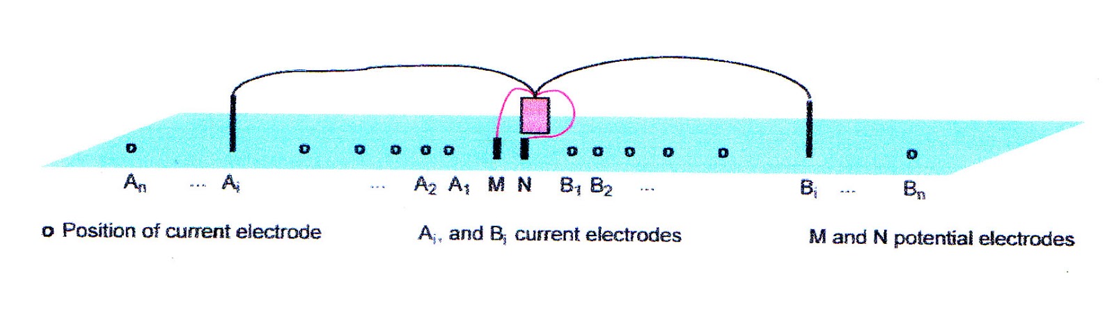
In electrode arrangement of SCHLUMBERGER m the geometric factor as follows :

K = 2 p/(1/AM – 1/AN) – (1/BM – 1/BN)  or

K = p{(AB)² – (MN)² } , where  AB=current electrode and MN=electrode  pot.

                    4 MN

  ρ =     KR = p{(AB)² – (MN)² }  R

                               4 MN

Figure 4. The electrode arranggement of SCHLUMBERGER     

In the SCHLUMBERGER method the electrode potential is fixed and will be change at certain distances. The maximum distance of AB/2 is not more than  5 x  MN/2.

2.2.2. The Relationship of Resistivity and Geology

Resistivity surveys give a picture of the subsurface resistivity distribution. To convert the resistivity picture into a geological picture, some knowledge of typical resistivity values for different types of subsurface materials of the area surveyed, of these rocks is greatly dependent is important.

Table 1 gives the resistivity values of  common rocks, soil materials and chemicals (Keller and Frischnecht 1966, Daniels and Alberty 1966 ). Igneous and metamorphic rocks typically have resistivity values. The resistivity of these rocks is greatly dependent on the degree of fracturing, and the percentage filled with ground water. Sedimentary rocks which usually are more porous and have a higher content, normally have lower resistivity values. Wet soills and fresh ground water have even lower resistivity values. Clayey soil normally has a lower resistivity value than sandy soil. However, note the overlap in the resistivity values of different classes of rocks  and soils. This is because the resistivity of a particular rock or soil sample depend on a number of factor such as porosity, the degreeof the watter saturation and the consentration of dissolved salt.

Table 1. Resistivity of some common rocks, mineral and chemical ( Keller and Frischnecht 1966 , Daniels and Alberty 1966 )

Material	Resistivity (ohm-m)	Conductivity (Siemen/m)
Igneous and  Metamorphic Rock -. Granite -. Basalt _. Slate -. Marble -. Quarzite	5 X 103 - 106 103 – 106 6x102 – 4x107 102 -  2.5 x 108 102 – 2x108	10-6- 2x10-4 10-6- 10-3 2,5 x10-8 – 1,7 x10-3 4 x 10-9 – 10-2 5 x 10-9 – 10-2
Sedimentary Rocks -. Sandston -. Limestone	8 – 4x 103 20 – 2x103 50 – 4x103	2,5 x 10-4 – 0,125 5.10-4 – 0,05 2,5 x 10-3 – 0,02
Soils and Water -. Clay -. Alluvium -. Groundwater (fresh) -. Sea Water	1 – 100 10 – 800 10 –100 0,2	0,01 – 1 1,25 x10-3 – 0,1 0,01 – 0,1 5
Chemicals -. Iron (Fe) -. 0,01 M Potassium Chloride -.0,01 M Sodium chloride -.0,01 M acetic acid -. Xylene	9,07x 10-8 0,708 0,843 6,13 6,998 x 1016	1,102 x107 1,413 1,183 0,163 1,429 x 10-17

The resistivity of ground water varies from 10 to  100 ohm-mm depending on the concentration of  dissolved salt. Note the low resistivity ( about 0.2 ohm-m of the sea water  due to the relatively high salt content. The value of resistivity related to the rock type and water quality shown on Figure 5.  

Generally, the hot water is came from the fresh water , which is through heating from underground or from heating of magma. The hot fluid from magma  transmit through fracture of base rocks.The heating of magma or rocks is boiled the fresh water become hot water, which estimated resistivity from 0.1 ohm-m to less than 10 ohm-m., which is depend of temperature water.

Figure 5. Relationship value of resistivity with groundwater quality ( salty, brackish and fresh ) and rocks types (Flathe H.,1979).

2.2.3.The Conventional Resistivity or Resistivity 1 D ( one Dimension )

The conventional resistivity or resistivity 1 D has its origin in the 1920’s due to the work of the Schlumberger brothers. At the same time, in USA  Wenner had introduced the electrode arrangement of Wenner.

The measured apparent resistivity values are normally plotted on a log-log graph paper and data interpreted using matching curves. It is assumed that the subsurface consists of horizontal layers.  In this case ,the subsurface resistivity changes only with depth,but does not change in the horizontal direction, as shown in Figure 6.

The software for data interpretation have been  made by several institution such as VESPC, RESINT 53, GRIVEL, IP2Win and RES 1D.

Figure 6. The electrode arrangement and datum points in the resistivity 1-D.

2.2.4. The Unconventional Resistivity or Resistivity 2 ( 2 dimension )

The greatest limitation of the resistivity sounding method is that does not take into account horizontal changes in the subsurface resistivity. A more accurate model of the subsurface is a two-dimensional ( 2-D) model where the resistivity changes in the vertical direction, as well as in the horizontal direction along the survey line. In this case , it is assumed that resistivity does not change in the direction that is perpendicular to the survey line. In many situation, particularly for survey over elongated geological bodies, this is a reasonable assumption. Typical 1-D resistivity sounding surveys usually involve about 10 to 20 readings, while 2-D imaging survey involve 100 to 1000 measurements.

The arrangement of electrode and the result of measurement shown on that we call the datum point. The figure 6 show the electrode arrangement and datum point in resistivity 2-D.

  

Figure 7. The electrode arrangement and datum points in resistivity 2-D.

The interpretation of data resistivity 2-D will be used the software RES2DINV. The RES2DINV has been introduced by Dr. H.M. Loke in 1997, 1999, 2000.  

3.       THE SHALLOW GEOTHERMAL AT MARGA MUKTI, PANGALENGAN KABUPATEN  
       BANDUNG SELATAN     

3..1. General.

Geoelectric soundings has been carried out in hot spring area of Desa Marga Mukti , Kecamatan Pangalengan, Kabupaten Bandung Selatan. The hot spring is one of the geothermal field in the areas. Currently ,the hot spring have been used for bathing for villagers. The hot spring is closed to the geothermal area which is located about 5 km at the western of G. Wayang.

Geothermal is meant that a total heat contained and collected in the earth to build geothermal system since the existed of the earth.  The geothermal system is similar to hydrothermal system, that is heating of groundwater or water collected in the under ground. The heating of water or geothermal system have several condition such us existing of water, hot rocks , permeable aquifer with high porosity  and the cap rocks to prevent of heat from the ground.

The geoelectric sounding carried out at the site into resistivity 1-D with the electrode array of Schlumberger and resistivity 2-D with Wenner-Schlumberger array with a = 10 m and the total electrode 50.

The location of the geoelectric sounding shown in Figure 8 The results of the resistivity 1-D  and  2-D shown in Figure 11 and Figure 12.

         

Figure 8. The Scheme of  g3oelectric soundings at tge hot spring of Desa Marga Mukti.

3.2. Topography and Geology

The location of sounding located on the elevation 1500 m  on the western of G, Wayang ( 2182m ). The area  is surroundings of mountain area such as G. Malabar ( 2321 m ) , G.  Guha ( 2391 m ) and G. Windu ( 2054 m ). The main river flows from the south to the north and joined with Citarum River at Nagreg.

The area shown on the Geological Map of Indonesia Sheet Garut an Pameungpeuk , Java scale 1 : 100.000. Geological description and geological condition have been done by M.Alzwar,et al (1992 ). According to M, Alzwar at all ( 1992 ) the oldest rocks  in this geological sheet is Benteng Formation in Upper Miocene in age.  Afterward the formation was un conformable with the younger rock formation. Than the rock unit covered with the youngest formation up to covered by Quaternary Rocks Formation.

The investigation area is covered with Undifferentiated Efflata Deposits of Young Volcanic (Qopu), which is  consist of volcanic ash, lapilli, sandy tuf and blocks andesite-basalt , laharic breccia and efflata.

The hydrogeological map of area indicated that groundwater condition have intermediate aquifer with wide distribution and the estimated discharge 10 l/sec. (Soetrisno S, 1983 ).

The geological and the hydrological map are shown in  Figure 8 and Figure 9

Figure 9. The Geological Map of Garut and Pameungpeuk, Jawa( M.Alzwar et all. 1992 )

Figure 10. The Hydrogeological Map of Sheet V Bandung ( Soetrisno S, 1983 }

3.3. Results of Geoelectric Sounding.

3.3.1.  Resistivity 1-D Schlumberger Array

The field data has been plotted to double log paper and run the data with using IP2Win. The data interpreted that the layer of resistivity existed for 4 to 6 layer at each sounding point. The result of running data was compare to the geological condition. Afterward, the resistivity 1-D section have been made through sounding point R 01, R 02 , R 03 , R 04 and R 05. The section of resistivity 1-D is shown on Figure 11.

The layers of resistivity had been group into 4 (four) layers. The first layer is value of resistivity from 1.60 ohm-m,54.57 ohm-m and 106 ohm-m and 989 ohm-m and interpreted as clay soil, sandy soil with boulder of rocks. The thickness of layer estimated 1 m to 2 m. The second layer is sandstone or volcanic sand with resistivity 24 ohm-m and 169 ohm-m with depth of 10 m to 40 m. The layer was divide into upper part and lower part separated with sand contained hot water. The third layer is sand or volcanic sand contained hot water with value of resistivity 4.09 ohm-m to 13.8 ohm-m. The four layer is the values of resistivity 700 ohm-m to 2715 ohm-m its interpreted as the volcanic rocks or base rock (see Figure 11 ).

Figure 11. The geology section of Resistivity 1-D electrode arrangement of SCHLUMBERGER AB/2 = 300 m.

3.3.2. Resistivity 2-D   Wenner-Schlumberger Array

The result of resistivity 2-D is devided into 4 (four  ) layer of resistivity. The first layer  clay soil, sandy soil and boulders. the with the value of resistivity 34,6 ohm-m, 163 ohm-m and 774 ohm-m. The thickness of layer estimated 1 m to 2 m.The second layer is volcanic sand or sandstone with the resistivity of 34.5 ohm-m to 163 ohm-m. The third layer located on the second layer indicated of hot water and inclusion of boulders. The sand of hot water has the value of resistivity 0.32 ohm-m to 7.3 ohm-m. Underneath of sandstone of second layer located the volcanic rock or base rock with the value of resistivity of 774 ohm-m to 17.000 ohm-m.   

The distribution of layer resistivity shown on Figure 12.

Figure 12. The Pseudosection of Resistivity 2-D Wenner - Schlumberger with a=10 m and Electrode  50,

2.       DISCUSSIONS

The area of geoelectric sounding covered by Undiferentiated Efflata Deposites of Young Volcanic ( Qopu ). The rock unit consists of volcanic ash, and lapili, sandy tuff, breccia of andesite-basalt, laharic breccia and efflata G. Wayang and its surroundings existed the 5 (five ) hot springs. One of the hot water has been used by PT. Pertamina – LEMIGAS, which it located on the foot of the hill of G.Wayang.

Generally, all of hot spring located on the stucture faulting. Its ration able, because the hot water flows through the faulting upward to the ground surfaces. It is also indicated that underneath of formation ( Qopu ) located fresh water bearing formation and the heating rocks underneath. That is approved that fresh water as shown on the hydrogeological map , that the discharge less than 10 l/sec.

On the site . there is existed hot spring which is indicated that the hot spring on the water bearing formation. The formation have been influent of faulting, so the hot water under pressure and reaches the ground surface. The water bearing formation on the area divided into  2 ( two ) conditions. Firstly, the water bearing formation on the heating rock will be changed of value of resistivity from 0.32 ohm-m to 7.3 ohm-m. The changed value of resistivity because the temperature high and viscosity of water low  and high of the ions mobility. However, on the other place the value of resistivity more than 34.5 ohm-m, it is indicated that the heating does not reach the formation. The heating  rocks have the value of resistivity of 700 ohm- to 17.000 ohm-m and interpreted as the base rock.

Figure 11 and Figure 12 shown that water bearing formation on the  middle of the section. However, the water bearing formation at 2 ( two ) places had been change to low resistivity, because of influency of heating rocks.  The thickness of hot water laying on the depth of 10 m to 60  m.

The further of investigation is to explore the hot water of the area.  Tt is recommended to drill on the sounding point with various depth, as follow  :

1.     Sounding point of R 01 with depth of 30 m. to 50 m.

2.     Sounding point of R 02 with depth of 50 m to 100 m.

3.     Sounding point of R 03 with depth of 40 m to 50 m.

4.     Sounding point of R 04 with depth of 50 m.

5.     Sounding point of R 05 with depth of 50 m to 60 m.

3.       CONCLUSION AND RECOMMENDATION

The area of survey and its surroundings is covered of Undiferentiated  Efflata Deposits of Young Volcanics ( Qypu ). This rock unit contained water bearing formation ( confined aquifer ) with the resistivity 24 ohm-m to 163 ohm-m. The water bearing formation was influent of hot fluid or heating rock at certain places and the resistivity become lower than origin. The value of resistivity 2-D was became 0.32 ohm-m to 7.00 ohm-m, its lower than resistivity 1-D was 4.09 ohm-m to 13.8 ohm-m.  The decrease of value of resistivity is caused the high temperature increase and a lower the viscosity and a high mobility of ions.

The exploration drilling should be done on the sounding points at the certain depth to exploit of the hot water.

It is recommended to make survey of geochemical of the hot spring and to measure hot water temperature.

It is recommended to construct the water collector, so the advantaged of hot water will be used soon.

REFFERENCES

1.     Orellana and Mooney, 1966, The Master Tables and Curves for Vertical Electric Sounding over  layered structures, Interciencia, Madrid.

2.     Flathe, H., 1979, The role of geologic concept in geophysical research works for solving hydro  geological problems. Geoexploration , 14 : 195 – 206.

3.    M. Alzwar drr., 1992, The Geological Map of Sheets Garut dan Pameungpeuk , Java Scala 1 :  100.00. P3G Bandung.

4.    Soetrisno S.,1983, The Hydrogeological Map Sheet  V Bandung, Scala 1 :250.000, Dit. GTL,  Bandung.

5.  Software of IP2Win, one program for interpretation of geo-electric data programmed by  University of Moscow.

6.   Keller and Frischknecht F.C.  1966. Electric Methods in Geophysical Prospecting, Pergamon  Press, New York, 519 pp.

7.     M.H. Loke, Dr. 1997,1999, 2000, Electrical Imaging surveys for environmental and engineering  studies. A practical guide in 2-D and 3-D surveys. Email : mhloke@pc.jarinf.my  and drmhloje@  hotmail.com

8.    Geotomo Software Malaysia, Juni 2011, Geoelectrical Imaging 2D and 3D, RES@DINV x 32  ver,3.71 with multy core support. RES2DINV x64 ver. 4.00  with 64- bit support. Rapid 2-D  Resistivity & IP inversion using the least-squares method.

9.   Idrus lhamid, 1982, Resistivity Survey of The Cisolok – Cisukarame Geothermal Authority  Grenssasvegor 9, 108 Rekjavik, ICELAND,UNU – GTP -1982 – 05 pdf fikle.